Early Synthesis
Although the synthesis of carbon nanotubes is almost 90 years old, it had gathered higher interest only when suitable measurements revealed the material’s nanoscale composition and astonishing photonic properties.
1930
From what we can say with today’s insights into synthesis conditions and techniques for the production of carbon nanotubes, the first report on a successful synthesis and confirmation of the nanostructure of the material was released in 1932 by Ulrich Hofmann from the Technical University of Berlin.[20][21] He worked with his father who by then had a research experience on graphitic carbon allotropes of more than ten years[22][23]. Hofmann et al. distinctively identified a new form of hexagonal carbon by looking at changes in the hexagonal crystal unit cells for different synthesis temperatures between 400℃ and 950℃.
Note
Besides using X-ray diffraction, hexagonal unit cells of graphitic carbon can be identified by Potassium K adsorption tests where calorimetrically three different adsorption states of Potassium per Carbon (16M, 8M, 4M) are identifiable.[24]
The structure was neither comparable to the lustrous graphenic form which forms on a substrate at 930℃ [25] nor to the black amorphous carbon structures that are found above 950℃. The new material was shown to form on iron, cobalt and nickel catalyst at 850℃ and 950℃. In their paper, they proposed a hexagonal prism with rounded edges as the unit cell. The diameter of this unit cell was measured to be 1.4nm at 850℃ and 1.7nm at 950℃ which is a reasonable mean carbon nanotube diameter for the used benzine precursor at these temperatures.
Note
A calculated roll-up angle for these structures would be 13° and 15° which is roughly the mean average of the theoretical minimum and maximum angle of carbon nanotubes.

A prismatic hexagonal unit cell with rounded edges as proposed by Hofmann et al. in 1932 is close to what we see as a nanotube today.
The electron microscope was invented in 1933 and became commercially available in 1938.[26] It is noteworthy that these early reports did not have access to this technique. Consequently, Hofmann analyzed the material that he synthesized in 1932 with this new microscopy technique almost ten years later in 1941 together with Manfred von Ardenne who is the inventor of transmission electron microscopy. In their report, they prove that the new material consists of chains of spherical carbon.[27] Later reports always show the existence of carbon nanotubes with electron microscopy, which shows that this fundamental visual technique opened insights into nanostructured graphitic carbon allotropes.
1950
As stated by Montieux[28], there had been earlier reports on the production of carbon filaments back unto 1889 but the main credit for “the discovery of carbon nanotubes” should go to Radushkevich and Lukyanovich [29] who published a series of rather detailed electron microscopy images in 1952. Regarding the research on the synthesis conditions, though, they cite some of the earlier German articles but not necessarily the relevant ones.
Although there had been previous reports [30], the first correct analysis for the growth conditions of carbon nanotubes in English speaking literature had been carried out in 1953 by W.R. Davis, R.J. Slawson, and G.R. Rigby [31]. Working for the British Research Association, they were intentionally investigating the disintegration of bricks in blast furnaces. In their report on a “minute vermicular [form of carbon]”, they correctly identified iron as the catalyst, carbon monoxide as the carbon source, and high temperatures (>450℃) for the growth of carbon nanotubes. At the time of writing, the research of Davis et al. was state of the art in electron microscopy working at the resolution limit of 10nm. Within the short report, they also suggested a growth mechanism that holds until today: They found that the catalyst particles are located at the end of the growing nanotubes and successive bundling takes place in the bulk raw material. Even though they underestimated the growth temperature by at least 150℃, this report is overly astonishing from today’s point of view as it identifies all necessary conditions for the synthesis of carbon nanotubes.
1960
How important the use of an electron microscope was, shows the first synthesis of carbon structures via chemical vapor deposition in 1959 [32]. Although, Walker et al. measured surface area and crystal structure, they were not able to report on nanostructures most likely due to the missing availability of microscopic methods.

Carbon Nanotubes consist of a graphitic hexagonal lattice. Its unit cell is
extended along the two hexagonal unit vectors to form a cylindircal object.
The picture shows the extension of the unit cell vectors  which is called a (6,5) carbon nanotube in
the commonly used Dresselhaus notation.
which is called a (6,5) carbon nanotube in
the commonly used Dresselhaus notation.
In 1960 Roger Bacon carried out the first comprehensive analysis on carbon filaments.[33] In his publication he collects different growth temperatures (350-1000℃) and extends the list of valuable catalysts to iron, cobalt, and nickel. Bacon uses arc-discharge on a graphitic electrode as a synthesis method with defined growth control. His key finding is the confirmation of the bent graphitic nature of the carbon lattice by Bragg diffraction. Due to their high length to diameter ratio, he named the filaments “Graphite Whiskers”. When describing the raw aggregated carbon nanotubes, he referred to “bundle[s] of Christmas tinsel”. In his attempt to explain the high resistivity against strain, he introduces a scroll-like structure. The carbon nanotubes should be rolled in a continuous helical spiral rather than in discrete cylinders.
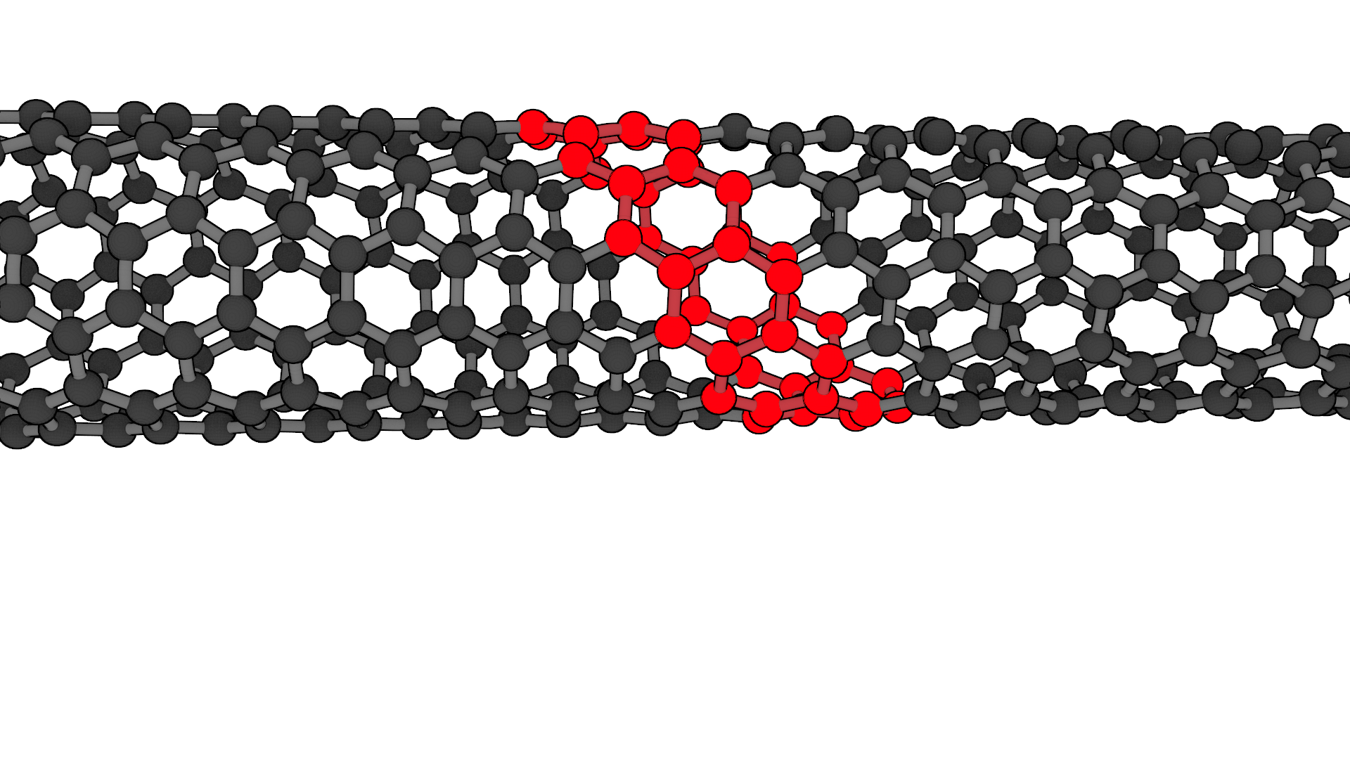
Rolling the graphene unit cell at an angle of 27° to the unit vector forms a (6,5) carbon nanotube.
Based on our knowledge today, these early publications were describing large bundles of carbon nanotubes, largely overestimating the diameter by one to five orders of magnitude. Nevertheless, those discoveries of a nano-scaled world are overly astonishing as the first electron microscope was constructed only 20 years before this discovery by Ruska at Siemens [26]. Despite the presence of suitable microscopic techniques and the knowledge about the proper synthesis conditions, research on carbon nanotubes became stale until the beginning of the early 1990s.
1990
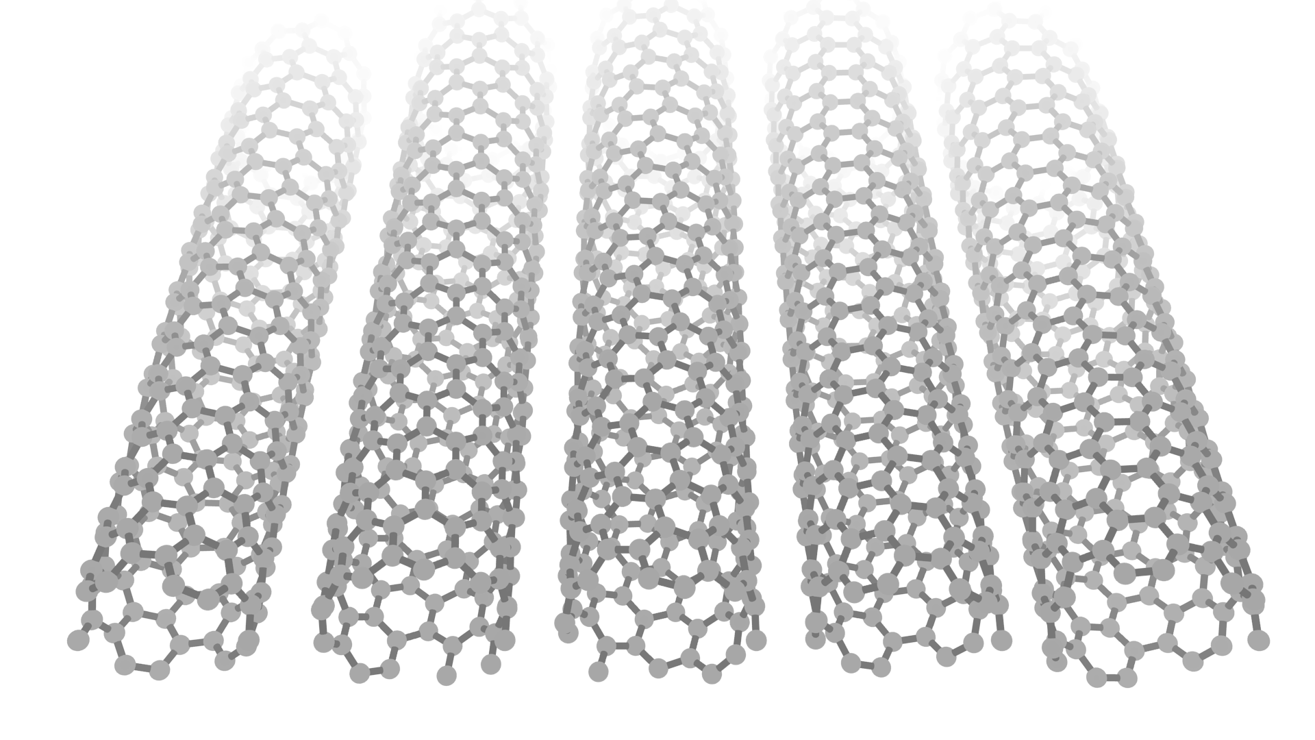
The (n,m) descriptor defines the unit cell extension.
Differently rolled carbon nanotubes with increasing diameters from 0.7nm to 0.9nm: LTR (6,4), (9,1), (8,3), (6,5), and (7,5) type.
Initially, the arc-discharge technique was used for the synthesis of C60 fullerenes in the middle of the 1980s [34]. This look into graphitic carbon nanostructures also revived research on carbon nanotubes: In the year 1991, Sumio Iijima described “needle-like” “microtubules”[35] as by-products during the synthesis of fullerenes. Using X-ray diffraction, he confirmed the previously mentioned findings by Bacon that the underlying hexagonal graphene lattice is indeed helically rolled up at a certain angle to the tube axis. In his attempt to confirm Bacon’s scroll model, he searched for overlapping edges at the outer surface of the “carbon needles” using transmission electron microscopy. As he was not able to find those features, he suggested concentric cylinders. Each tube should have spiral growth steps at the beginning and end similar to screw dislocations in a planar graphene lattice. With his publication, he not only correctly described multi-wall carbon nanotubes but also introduced discrete roll-up angels and pointed out that the screw dislocation produces handed (chiral) tubes.
Excitons

The charge-separated net-neutral state of an electron and a hole binds through quantum mechanical forces and forms quasi-particles that are called excitons.
Although the carbon nanotubes described in this initial report were multi-wall due to typical synthesis temperatures of 4000℃, it was readily after recognized by Riichiro Saito that single-wall carbon nanotubes of the described cylindrical structure would have unique electrical properties.[36]
Sumio Iijima also reported the first actual synthesis of single-wall carbon nanotubes (SWNT) only two years after his initial report on multi-wall carbon nanotubes.[37] Due to their rolled symmetry, the electronic bands in SWNT accumulate at distinct energy levels, which are called van-Hove singularities. These singularities allow charge-separated states to exist. Even though the Coulomb interaction acts attractive, the quantum mechanical exchange interaction allows these systems to form a bound state. The one-dimensional confinement in the tubular structure causes binding energies of up to 500meV, which allows these quasi-particles, so-called excitons, to be stable at room temperature. Ando et al. theoretically predicted excitons [38] and in 2005 they were also experimentally confirmed using 2-photon spectroscopy [39].
Chiral Distribution

Nanotubes can have the same diameter as can be seen for the (6,5) and (9,1) type, but only the roll-up angle defines their distinct electronic band structure. Plotting the diameter of a carbon nanotube against its energy separation between first and second subbands is called a Kataura plot[40].
Data for this Kataura plot was measured in air by Liu et al.[41]
More control over the synthesis process with higher yields and overall smaller diameters was first achieved in 1995 by laser ablation or laser furnace techniques.[42][43][44] There have also been routes for the deposition in plasmas generated by solar furnaces, but there is generally no need for going to such high temperatures during synthesis.[45][46] All of these techniques produce bundles [47] and chiral distributions with a larger mean diameter. Other innovative approaches use wet chemical synthesis to construct single chiral samples from the bottom up using Scholl reaction or aryl-aryl domino coupling.[48][49][50] A more cost-effective production environment that gives good control over the diameter distribution and also allows up-scaling to commercial production grades[51] is chemical vapor deposition.
Conclusion
Without going into more detail of the early advances in carbon nanotube synthesis, it should be clear by now that it is crucial to control both synthesis and analysis methods to investigate a new material properly. In the following chapter I want to concentrate on chemical vapor deposition as the preferred synthesis technique in this study to create samples of single-wall carbon nanotubes with diameters between 0.7 and 0.9nm and a length of 2µm and more on different substrates. Advances in optical techniques also allow doing more thorough analyses than what is possible with electron microscopy. The following chapters will introduce the synthesis technique to produce the samples and the principal optical characterization methods for taking images and spectra.